By default, every row and column of a new workbook is set to the same height and width. Excel allows you to modify column width and row height in different ways, including wrapping text and merging cells.
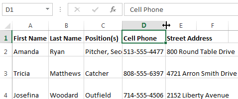
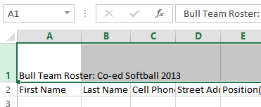
In our example below, some of the content in column A cannot be displayed. We can make all of this content visible by changing the width of column A.
Position the mouse over the column line in the column heading so the white cross becomes a double arrow.
Hovering over the column line
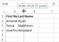
Click, hold, and drag the mouse to increase or decrease the column width.
Increasing the column width
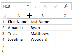
Release the mouse. The column width will be changed.
The new column width
If you see pound signs (#######) in a cell, it means the column is not wide enough to display the cell content. Simply increase the column width to show the cell content.
To AutoFit column width:
The AutoFit feature will allow you to set a column's width to fit its content automatically.
Position the mouse over the column line in the column heading so the white cross becomes a double arrow.
Hovering the mouse over the column line
Double-click the mouse. The column width will be changed automatically to fit the content.
The automatically sized column
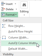
You can also AutoFit the width for several columns at the same time. Simply select the columns you want to AutoFit, then select the AutoFit Column Width command from the Format drop-down menu on the Home tab. This method can also be used for row height.
AutoFitting columns width with the Format command
To modify row height:
Position the cursor over the row line so the white cross becomes a double arrow.
Hovering the mouse over the row line
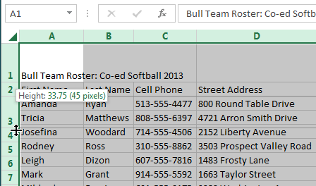
Click, hold, and drag the mouse to increase or decrease the row height.
Increasing the row height
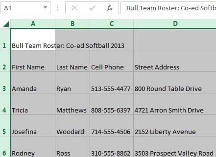
Release the mouse. The height of the selected row will be changed.
The new row height
To modify all rows or columns:
Rather than resizing rows and columns individually, you can modify the height and width of every row and column at the same time. This method allows you to set a uniform size for every row and column in your worksheet. In our example, we will set a uniform row height.
Locate and click the Select All button just below the formula bar to select every cell in the worksheet.
Selecting every cell in a worksheet
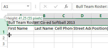
Position the mouse over a row line so the white cross becomes a double arrow.
Click, hold, and drag the mouse to increase or decrease the row height.
Modifying the height of all rows
Release the mouse when you are satisfied with the new row height for the worksheet.
The uniform row height
Inserting, deleting, moving, and hiding rows and columns
After you've been working with a workbook for a while, you may find that you want to insert new columns or rows, delete certain rows or columns, move them to a different location in the worksheet, or even hide them.
To insert rows:
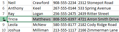
Select the rowheading below where you want the new row to appear. For example, if you want to insert a row between rows 7 and 8, select row 8.
Selecting a row
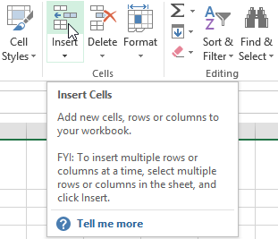
Click the Insert command on the Home tab.
Clicking the Insert command
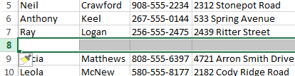
The new row will appear above the selected row.
The new row
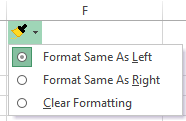
When inserting new rows, columns, or cells, you will see the Insert Options button next to the inserted cells. This button allows you to choose how Excel formats these cells. By default, Excel formats inserted rows with the same formatting as the cells in the row above. To access more options, hover your mouse over the Insert Options button, then click the drop-down arrow.
The Insert Options button
To insert columns:
Select the columnheading to the right of where you want the new column to appear. For example, if you want to insert a column between columns D and E, select column E.
Selecting a column
Click the Insert command on the Home tab.
Clicking the Insert command
The new column will appear to the left of the selected column.
The new column
When inserting rows and columns, make sure you select the entire row or column by clicking the heading. If you select only a cell in the row or column, the Insert command will only insert a new cell.
To delete rows:
It's easy to delete any row that you no longer need in your workbook.
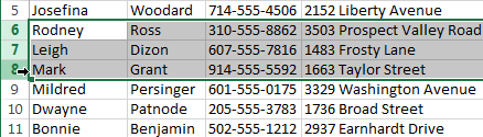
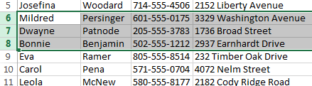
Select the row(s) you want to delete. In our example, we'll select rows 6-8.
Selecting rows to delete
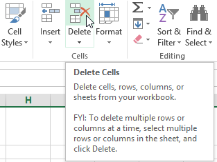
Click the Delete command on the Home tab.
Clicking the Delete command
The selected row(s) will be deleted, and the rows below will shift up. In our example, rows 9-11 are now rows 6-8.
Rows 9-11 shifted up to replace rows 6-8
To delete columns:
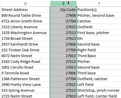
Select the columns(s) you want to delete. In our example, we'll select column E.
Selecting a column to delete
Click the Delete command on the Home tab.
Clicking the Delete command
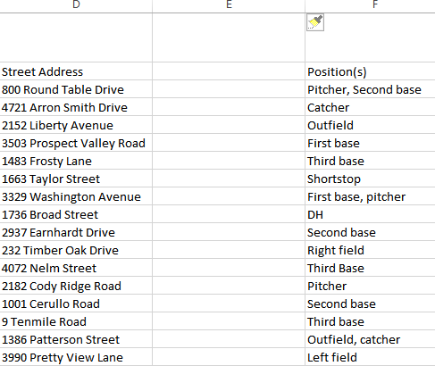
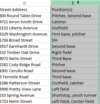
The selected columns(s) will be deleted, and the columns to the right will shift left. In our example, Column F is now Column E.
Column F shifted right to replace column E
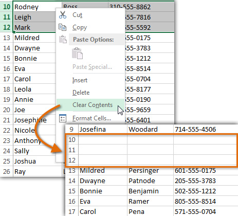
It's important to understand the difference between deleting a row or column and simply clearingits contents. If you want to remove the content of a row or column without causing others to shift, right-click a heading, then select Clear Contents from the drop-down menu.
Clearing the contents from several rows
To move a row or column:
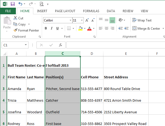
Sometimes you may want to move a column or row to rearrange the content of your worksheet. In our example we'll move a column, but you can move a row in the same way.
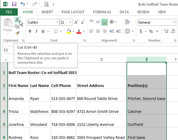
Select the desired column heading for the column you want to move, then click the Cut command on the Home tab or press Ctrl+X on your keyboard.
Cutting an entire column
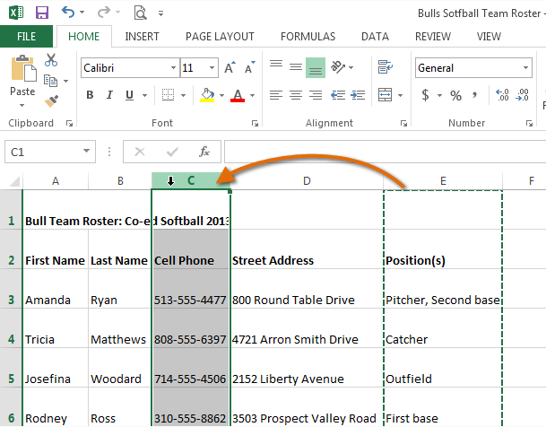
Select the columnheading to the right of where you want to move the column. For example, if you want to move a column between columns B and C, select column C.
Choosing a destination for the column
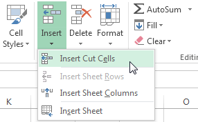
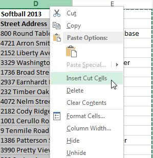
Click the Insert command on the Home tab, then select Insert Cut Cells from the drop-down menu.
Inserting the column
The column will be moved to the selected location, and the columns to the right will shiftright.
The moved column
You can also access the Cut and Insert commands by right-clicking the mouse and then selecting the desiredcommands from the drop-down menu.
Right-clicking to Insert Cut Cells
To hide and unhide a row or column:
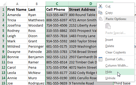
At times, you may want to compare certain rows or columns without changing the organization of your worksheet. Excel allows you to hide rows and columns as needed. In our example, we'll hide columns C and D to make it easier to compare columns A, B, and E.
Select the column(s) you want to hide, right-click the mouse, then select Hide from the formatting menu.
Hiding the selected columns
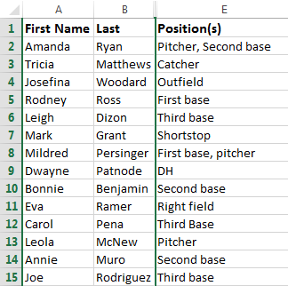
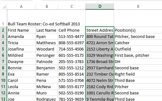
The columns will be hidden. The green column line indicates the location of the hidden columns.
The hidden columns
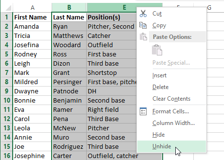
To unhide the columns, select the columns to the left and right of the hidden columns (in other words, the columns on bothsides of the hidden columns). In our example, we'll select columns B and E.
Right-click the mouse, then select Unhide from the formatting menu. The hidden columns will reappear.
Unhiding the hidden columns
Wrapping text and merging cells
Whenever you have too much cell content to be displayed in a single cell, you may decide to wrap the text or merge the cell rather than resize a column. Wrapping the text will automatically modify a cell's row height, allowing cell contents to be displayed on multiple lines. Merging allows you to combine a cell with adjacent empty cells to create one large cell.
To wrap text in cells:
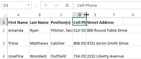
In our example below, we'll wrap the text of the cells in column D so the entire address can be displayed.
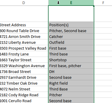
Select the cells you want to wrap. In this example, we'll select the cells in column D.
Selecting cells to wrap
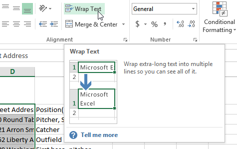
Select the Wrap Text command on the Home tab.
Clicking the Wrap Text command
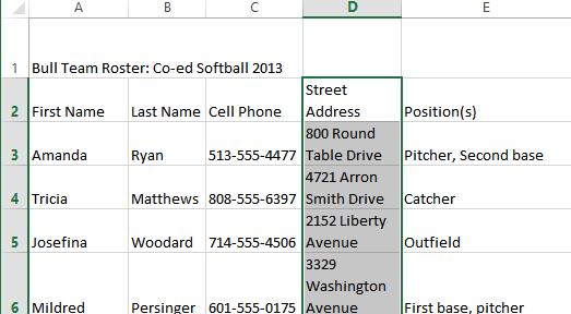
The text in the selected cells will be wrapped.
The wrapped text
Click the Wrap Text command again to unwrap the text.
To merge cells using the Merge & Center command:
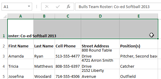
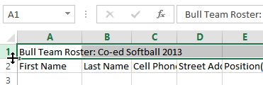
In our example below, we'll merge cell A1 with cells B1:E1 to create a title heading for our worksheet.
Select the cell range you want to merge.
Selecting cell range A1:E1
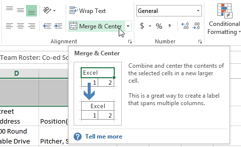
Select the Merge & Center command on the Home tab.
Clicking the Merge & Center command
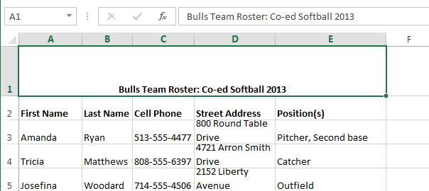
The selected cells will be merged, and the text will be centered.
Cell A1 after merging with B1:E1
To access more merge options:
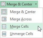
Click the drop-down arrow next to the Merge & Center command on the Home tab. The Merge drop-down menu will appear. From here, you can choose to:
Merge & Center: Merges the selected cells into one cell and centers the text
Merge Across: Merges the selected cells into larger cells while keeping each row separate
Merge Cells: Merges the selected cells into one cell but does not center the text
Unmerge Cells: Unmerges selected cells
Accessing more Merge options
Although merging cells can be useful, it can also cause problems with some spreadsheets. Watch the video below to learn about some of the problems with merging cells.
Challenge!
Open an existing Excel 2013 workbook. If you want, you can use our practice workbook.
Modify the width of a column. If you are using the example, use the column that contains the players' first names.
Insert a column between column A and column B, then insert a row between row 3 and row 4.
Delete a column or a row.
Move a column or row.
Try using the TextWrap command on a cell range. If you are using the example, wrap the text in the column that contains street addresses.
Try merging some cells. If you are using the example, merge the cells in the title row using the Merge & Center command (cell range A1:E1).


 becomes a double arrow
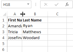
 .
.
 just below the formula bar to select every cell in the worksheet.
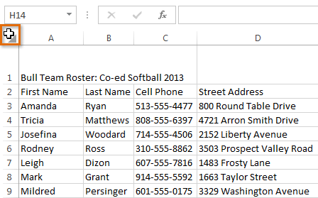
 next to the inserted cells. This button allows you to choose how Excel formats these cells. By default, Excel formats inserted rows with the same formatting as the cells in the row above. To access more options, hover your mouse over the Insert Options button, then click the drop-down arrow.