
Excel 2013 -
Cell Basics

Excel 2013
Cell Basics

search
menu
/en/excel2013/saving-and-sharing-workbooks/content/
Whenever you work with Excel, you'll enter information—or content—into cells. Cells are the basic building blocks of a worksheet. You'll need to learn the basics of cells and cell content to calculate, analyze, and organize data in Excel.
Optional: Download our practice workbook.
Every worksheet is made up of thousands of rectangles, which are called cells. A cell is the intersection of a row and a column. Columns are identified by letters (A, B, C), while rows are identified by numbers (1, 2, 3).
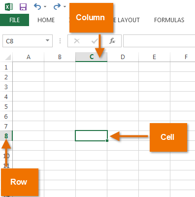 A cell
Each cell has its own name—or cell address—based on its column and row. In this example, the selected cell intersects column C and row 5, so the cell address is C5. The cell address will also appear in the Name box. Note that a cell's column and row headings are highlighted when the cell is selected.
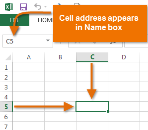 Cell C5
You can also select multiple cells at the same time. A group of cells is known as a cell range. Rather than a single cell address, you will refer to a cell range using the cell addresses of the first and last cells in the cell range, separated by a colon. For example, a cell range that included cells A1, A2, A3, A4, and A5 would be written as A1:A5.
In the images below, two different cell ranges are selected:
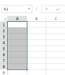 Cell range A1:A8
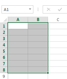 Cell range A1:B8
If the columns in your spreadsheet are labeled with numbers instead of letters, you'll need to change the default reference style for Excel. Review our Extra on What are Reference Styles? to learn how.
To input or edit cell content, you'll first need to select the cell.
 will appear around the selected cell, and the column heading and row heading will be highlighted. The cell will remain selected until you click another cell in the worksheet.
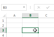 Selecting a single cell
You can also select cells using the arrow keys on your keyboard.
Sometimes you may want to select a larger group of cells, or a cell range.
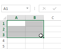 Selecting a cell range
Any information you enter into a spreadsheet will be stored in a cell. Each cell can contain different types of content, including text, formatting, formulas, and functions.
 Cell text
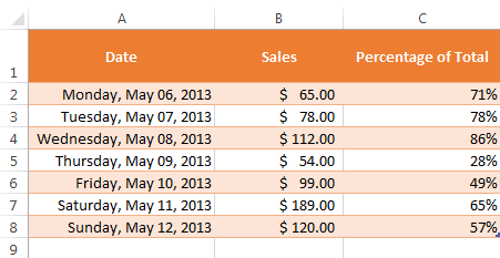 Cell formatting
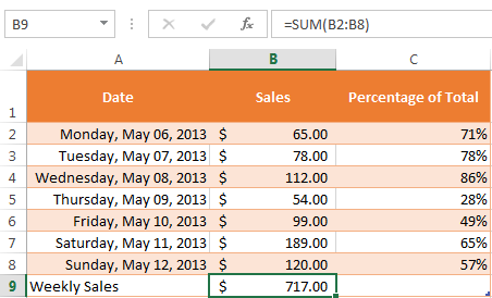 Cell formulas
 Selecting cell A1
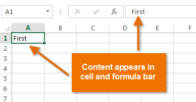 Inserting cell content
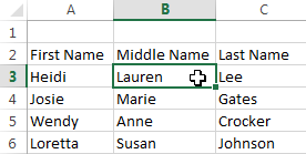 Selecting a cell
 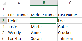 Deleting cell content
You can use the Delete key on your keyboard to delete content from multiple cells at once. The Backspace key will only delete one cell at a time.
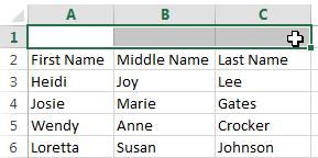
There is an important difference between deleting the content of a cell and deleting the cell itself. If you delete the entire cell, the cells below it will shift up and replace the deleted cells.
 Selecting a cell to delete
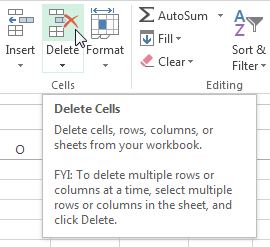 Clicking the Delete command
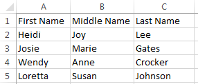 Cells shifted to replace the deleted cell
Excel allows you to copy content that is already entered into your spreadsheet and paste that content to other cells, which can save you time and effort.
 Selecting a cell to copy
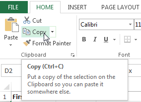 Clicking the Copy command
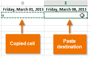 Pasting cells
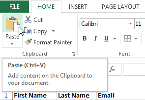 Clicking the Paste command
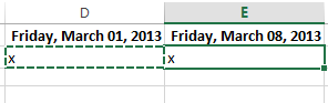 The pasted cell content
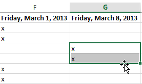
Unlike copying and pasting, which duplicates cell content, cutting allows you to move content between cells.
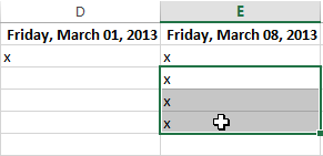 Selecting a cell range to cut
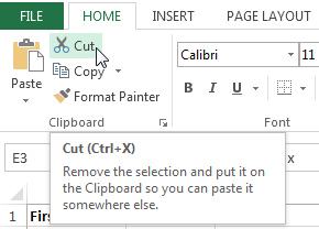 Clicking the Cut command
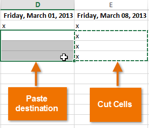 Pasting cellsClicking the Paste command
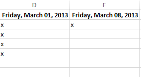 The cut and pasted cells
You can also access additional paste options, which are especially convenient when working with cells that contain formulas or formatting.
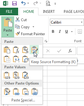 Additional Paste options
Rather than choose commands from the Ribbon, you can access commands quickly by right-clicking. Simply select the cell(s) you want to format, then right-click the mouse. A drop-down menu will appear, where you'll find several commands that are also located on the Ribbon.
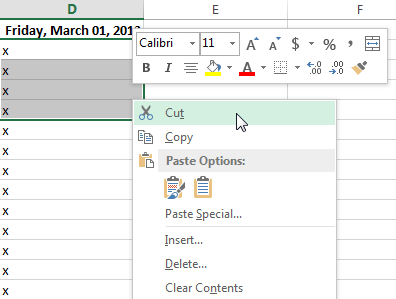 Right-clicking to access formatting options
Rather than cutting, copying, and pasting, you can drag and drop cells to move their contents.
 to a black cross with four arrows
 .
. Hovering over the cell border
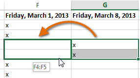 Dragging the selected cells
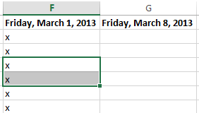 The dropped cells
There may be times when you need to copy the content of one cell to several other cells in your worksheet. You could copy and paste the content into each cell, but this method would be time consuming. Instead, you can use the fill handle to quickly copy and paste content to adjacent cells in the same row or column.
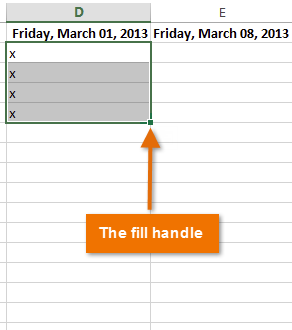 Locating the fill handle
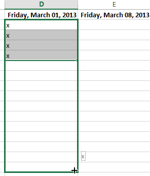 Dragging the fill handle
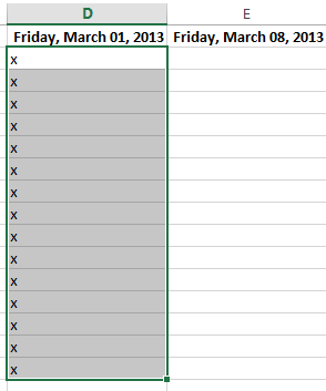 The filled cells
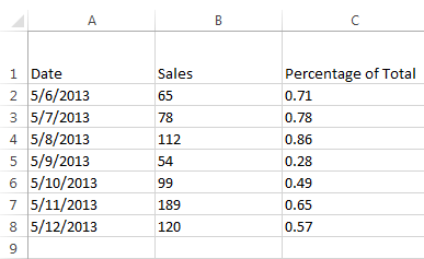
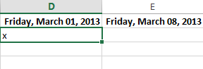
The fill handle can also be used to continue a series. Whenever the content of a row or column follows a sequential order, like numbers (1, 2, 3) or days (Monday, Tuesday, Wednesday), the fill handle can guess what should come next in the series. In many cases, you may need to select multiple cells before using the fill handle to help Excel determine the series order. In our example below, the fill handle is used to extend a series of dates in a column.
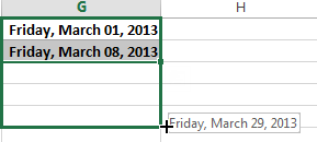 Using the fill handle to extend a series
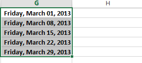 The extended series
You can also double-click the fill handle instead of clicking and dragging. This can be useful with larger spreadsheets, where clicking and dragging may be awkward.
Watch the video below to see an example of double-clicking the fill handle.
A new feature in Excel 2013, Flash Fill can enter data automatically into your worksheet, saving you time and effort. Just like the fill handle, Flash Fill can guess what type of information you're entering into your worksheet. In the example below, we'll use Flash Fill to create a list of first names using a list of existing email addresses.
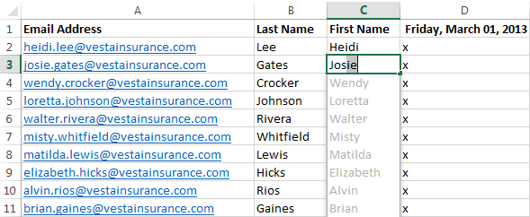 Previewing Flash Fill data
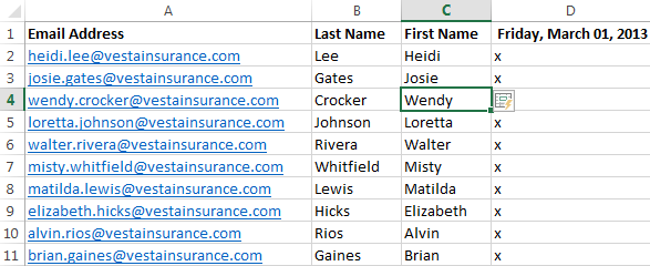 The entered Flash Fill data
To modify or undo Flash Fill, click the Flash Fill button next to recently added Flash Fill data.
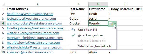 Clicking the Flash Fill button
When working with a lot of data in Excel, it can be difficult and time consuming to locate specific information. You can easily search your workbook using the Find feature, which also allows you to modify content using the Replace feature.
In our example, we'll use the Find command to locate a specific name in a long list of employees.
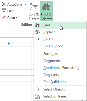 Clicking the Find command
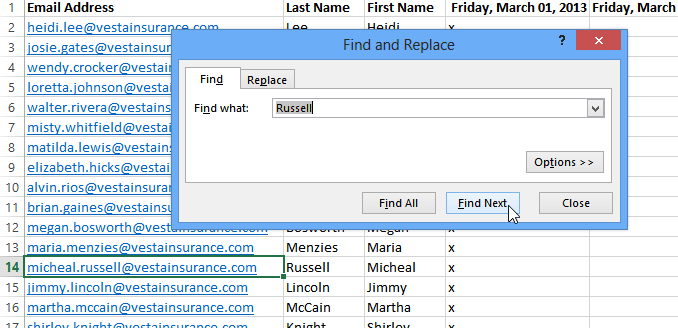 Clicking Find Next
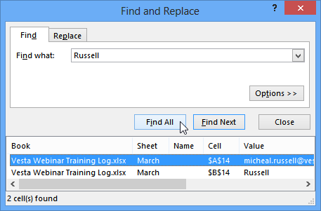 Clicking Find All
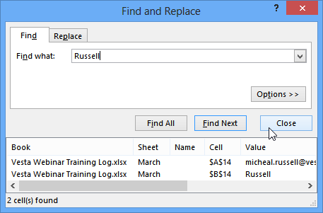 Closing the Find and Replace dialog box
You can also access the Find command by pressing Ctrl+F on your keyboard.
Click Options to see advanced search criteria in the Find and Replace dialog box.
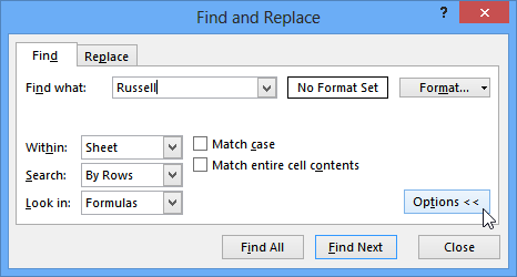 Clicking Options
At times, you may discover that you've repeatedly made a mistake throughout your workbook (such as misspelling someone's name), or that you need to exchange a particular word or phrase for another. You can use Excel's Find and Replace feature to make quick revisions. In our example, we'll use Find and Replace to correct a list of email addresses.
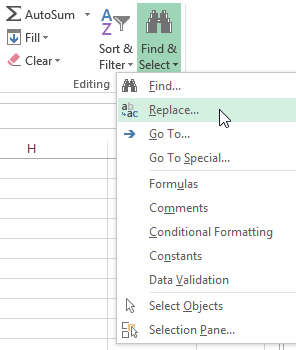 Clicking the Replace command
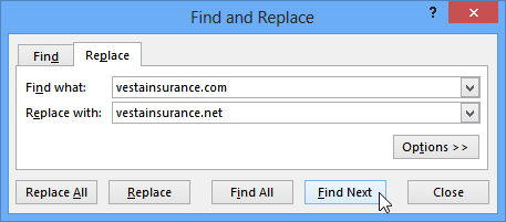 Clicking Find Next
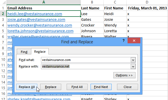 Replacing the highlighted text
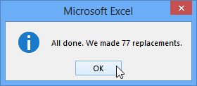 Clicking OK
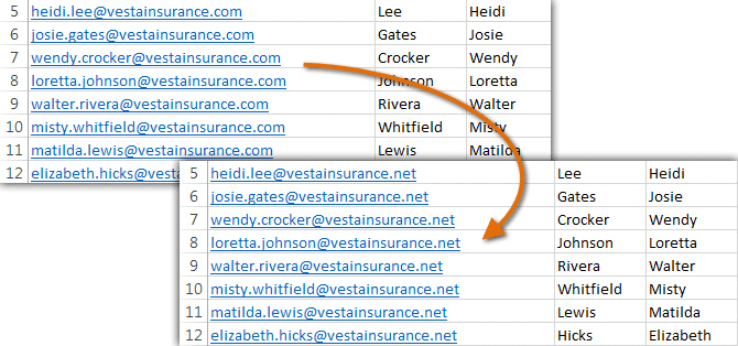 The replaced content
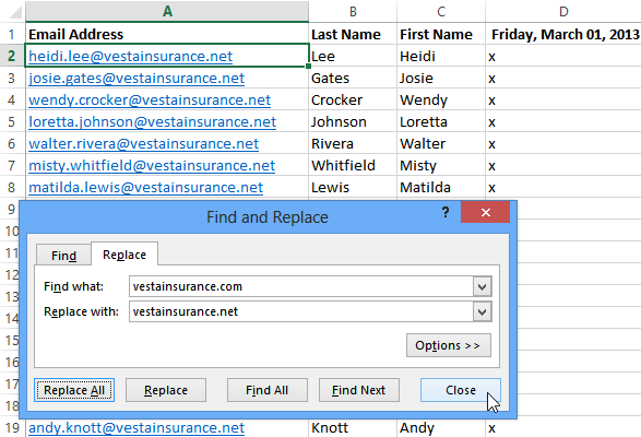 Closing the Find and Replace dialog box
/en/excel2013/modifying-columns-rows-and-cells/content/