/en/excel-tips/how-to-make-charts-auto-update/content/

Use Transpose to flip data on its side

Suppose you have a spreadsheet that is arranged into two rows, like the example below:

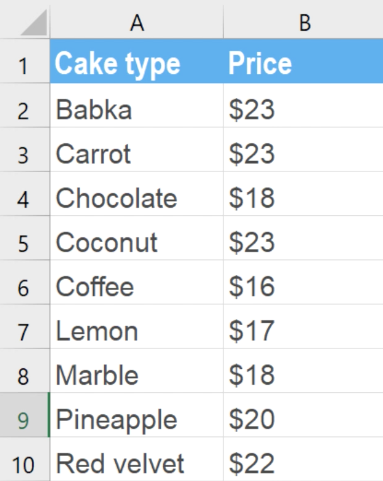
 This arrangement would quickly become unwieldy if more columns were added. It would be better to rearrange this data into two columns instead:

Luckily, you don't have to rearrange each cell by hand. Excel can do it automatically using a feature called Transpose, which is available when copying and pasting data.

Check out the video below to learn how to transpose data.

Steps

1. Select the data you want to flip on its side, including the headers. 
2. Press Ctrl+C to copy the data.
3. Right-click on a cell where you want to paste the transposed data. This cell needs to be somewhere outside of your original selection.
4. Under Paste Options, select Transpose.
5. The data will be pasted into the selected cell in a transposed format.
6. Delete the original data, if necessary.

Though you might not use this feature every day, it can help to rearrange your data into a format that’s easier to read. In Lesson 14, we’ll talk a little bit about absolute references. 

/en/excel-tips/absolute-references-with-the-f4-key/content/