/en/tr_ar-excel-2016/groups-and-subtotals-/content/

المقدمة

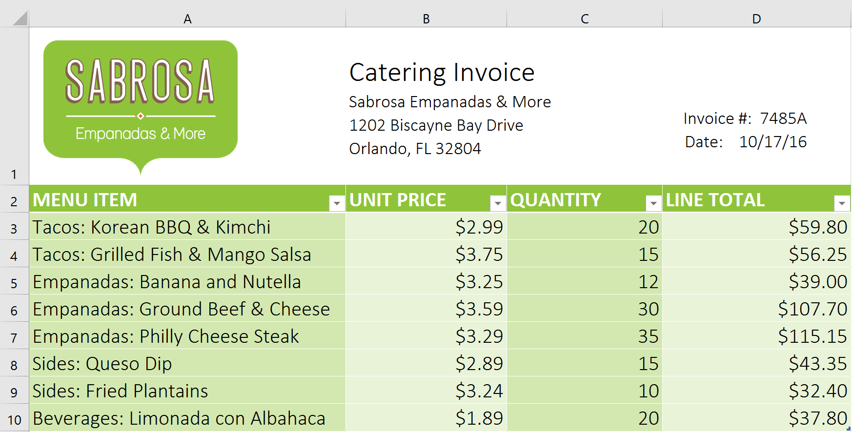
Once you've entered information into your worksheet, you may want to format your data as a table. Just like regular formatting, tables can improve the look and feel of your workbook, and they'll also help you organize your content and make your data easier to use. Excel includes several tools and predefined table styles, allowing you to create tables quickly and easily.

اختياري: تحميل ملف للتمرين .

Watch the video below to learn more about working with tables.

To format data as a table:

1. Select the cells you want to format as a table. In our example, we'll select the cell range A2:D9.
   
2. From the Home tab, click the Format as Table command in the Styles group.
   
3. Select a table style from the drop-down menu.
   
4. A dialog box will appear, confirming the selected cell range for the table.
5. If your table has headers, check the box next to My table has headers, then click OK.
   
6. The cell range will be formatted in the selected table style.
   

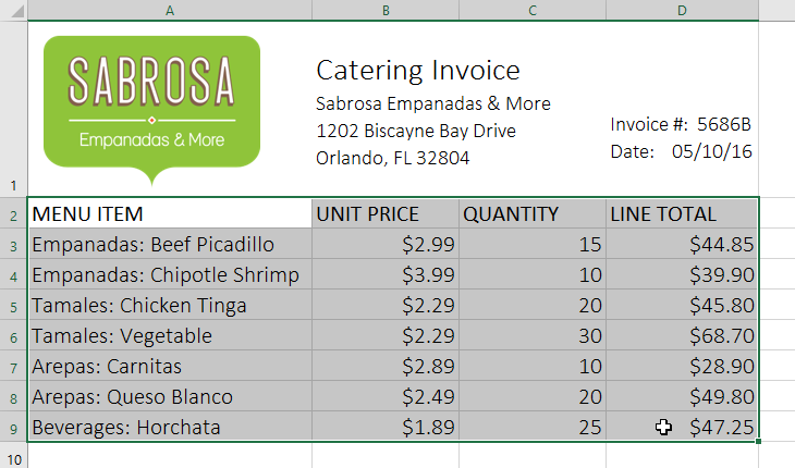
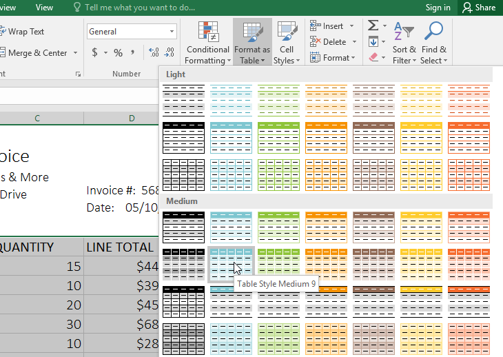
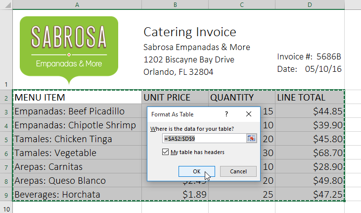
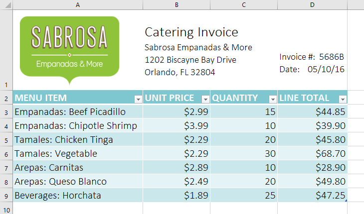
Tables include filtering by default. You can filter your data at any time using the drop-down arrows in the header cells. To learn more, review our lesson on Filtering Data.

Modifying tables

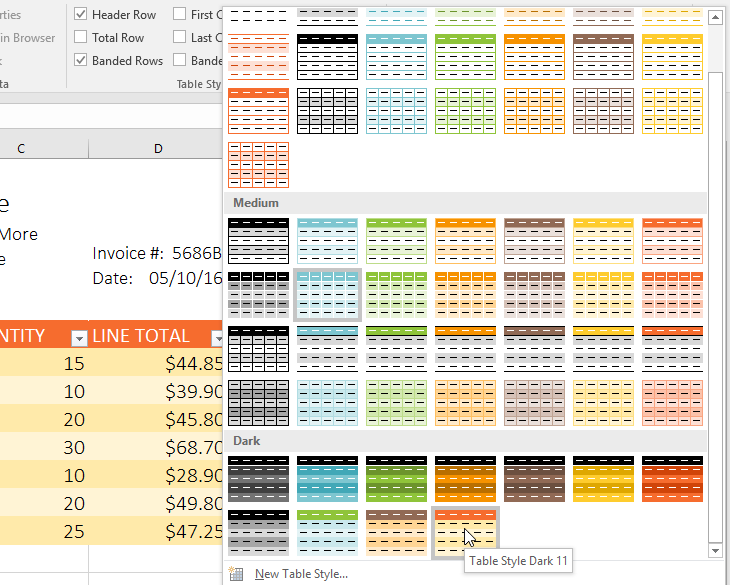
It's easy to modify the look and feel of any table after adding it to a worksheet. Excel includes many different options for customizing a table, including adding rows or columns and changing the table style.

To add rows or columns to a table:

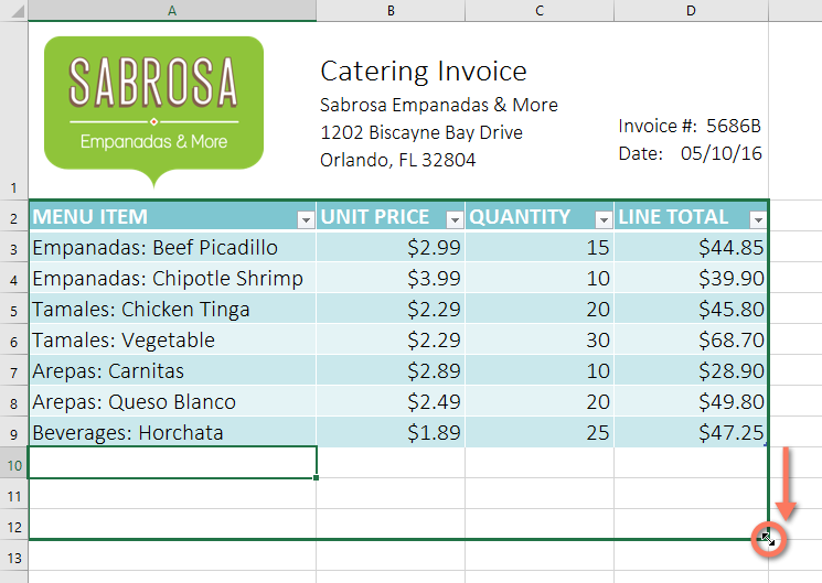
If you need to fit more content into your table, Excel allows you to modify the table size by including additional rows and columns. There are two simple ways to change the table size:

• Enter new content into any adjacent row or column. The row or column will be roped into the table automatically.
  
• Click and drag the bottom-right corner of the table to create additional rows or columns.
  

To change the table style:

1. Select any cell in your table, then click the Design tab.
   
2. Locate the Table Styles group, then click the More drop-down arrow to see all available table styles.
   
3. Select the desired table style.
   
4. The table style will be applied.

   

To modify table style options:

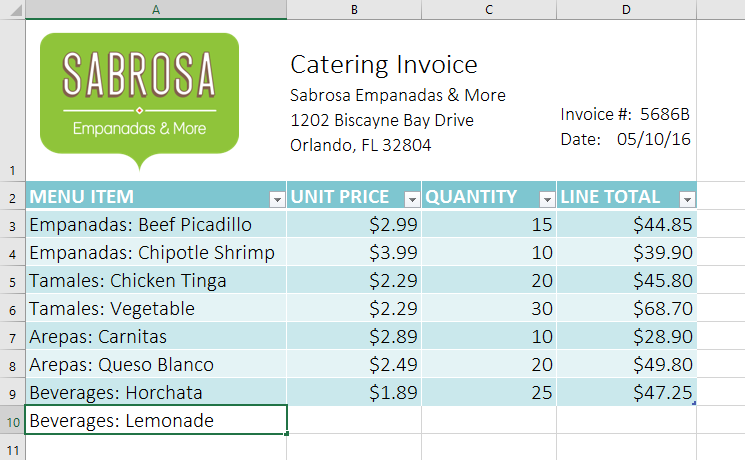
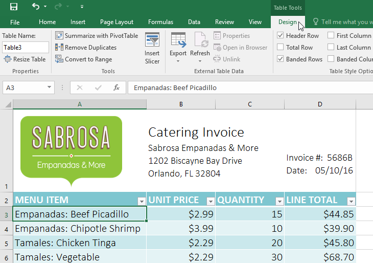
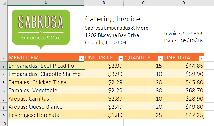
You can turn various options on or off to change the appearance of any table. There are six options: Header Row, Total Row, Banded Rows, First Column, Last Column, and Banded Columns.

1. Select any cell in your table, then click the Design tab.
2. Check or uncheck the desired options in the Table Style Options group. In our example, we'll check Total Row to automatically include a total for our table.
   
3. The table style will be modified. In our example, a new row has been added to the table with a formula that automatically calculates the total value of the cells in column D.
   

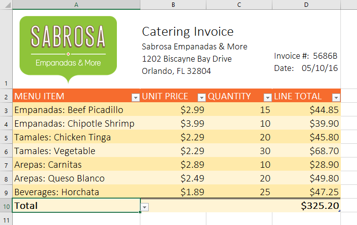
Depending on the type of content you have and the table style you've chosen these options can affect your table's appearance in various ways. You may need to experiment with a few different options to find the exact style you want.

To remove a table:

It's possible to remove a table from your workbook without losing any of your data. However, this can cause issues with certain types of formatting, including colors, fonts, and banded rows. Before you use this option, make sure you're prepared to reformat your cells if necessary.

1. Select any cell in your table, then click the Design tab.
2. Click the Convert to Range command in the Tools group.
   
3. A dialog box will appear. إنقر فوق Yes.
   
4. The range will no longer be a table, but the cells will retain their data and formatting.
   

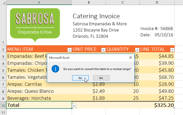
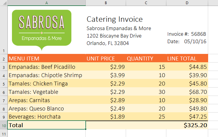
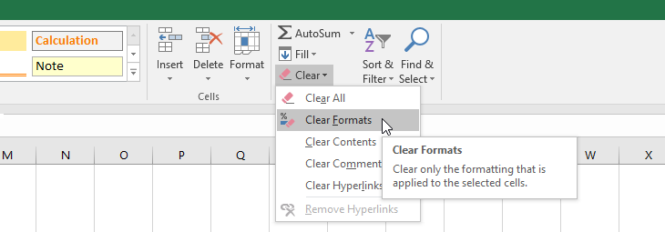
To restart your formatting from scratch, click the Clear command on the Home tab. Next, choose Clear Formats from the menu.

التحدي 3:

1. Open our practice workbook.
2. Click the Challenge tab in the bottom-left of the workbook.
3. Select cells A2:D9 and format as table. Choose one of the light styles.
4. Insert a row between rows 4 and 5. In the row you just created, type Empanadas: Banana and Nutella, with a unit price of $3.25, and a quantity of 12.
5. Change the table style to Table Style Medium 10.
6. In Table Style Options, uncheck banded rows and check banded columns.
7. When you're finished, your workbook should look like this:

   

/en/tr_ar-excel-2016/charts-/content/