
Excel 2013 -
Groups and Subtotals

Excel 2013
Groups and Subtotals

search
menu
/en/excel2013/filtering-data/content/
Worksheets with a lot of content can sometimes feel overwhelming and even become difficult to read. Fortunately, Excel can organize data in groups, allowing you to easily show and hide different sections of your worksheet. You can also summarize different groups using the Subtotal command and create an outline for your worksheet
Optional: Download our practice workbook.
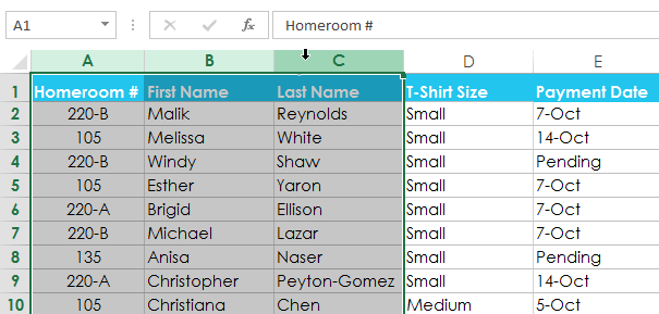 Selecting columns to group
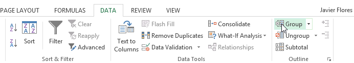 Clicking the Group command
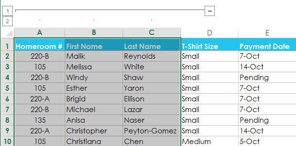 The grouped columns
To ungroup data, select the grouped rows or columns, then click the Ungroup command.
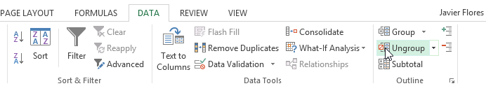 Clicking the Ungroup command
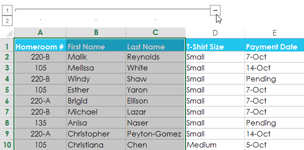 Hiding a group
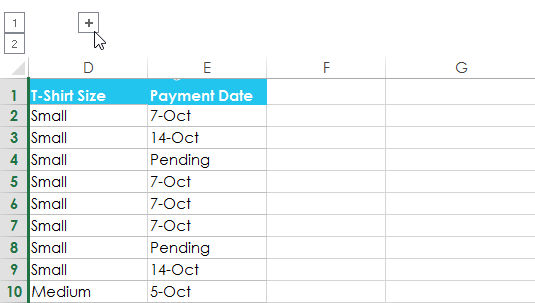 Clicking the Show Detail button to show the hidden group
The Subtotal command allows you to automatically create groups and use common functions like SUM, COUNT, and AVERAGE to help summarize your data. For example, the Subtotal command could help to calculate the cost of office supplies by type from a large inventory order. It will create a hierarchy of groups, known as an outline, to help organize your worksheet.
Your data must be correctly sorted before using the Subtotal command, so you may want to review our lesson on Sorting Data to learn more.
In our example, we will use the Subtotal command with a T-shirt order form to determine how many T-shirts were ordered in each size (Small, Medium, Large, and X-Large). This will create an outline for our worksheet with a group for each T-shirt size and then count the total number of shirts in each group.
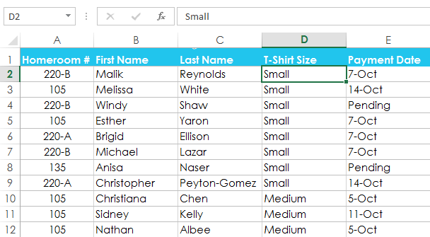 The worksheet sorted by t-shirt size
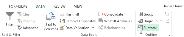 Clicking the Subtotal command
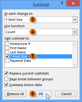 Creating a subtotal
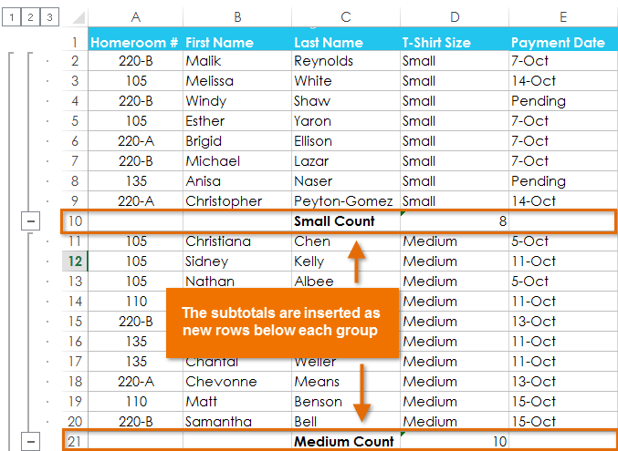 The outlined and subtotaled data
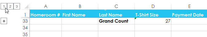
When you create subtotals, your worksheet it is divided into different levels. You can switch between these levels to quickly control how much information is displayed in the worksheet by clicking the Level buttons  to the left of the worksheet. In our example, we'll switch between all three levels in our outline. While this example contains only three levels, Excel can accommodate up to eight.
 Viewing data at the lowest level
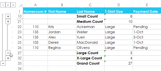
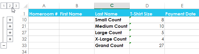 Viewing data at the next level
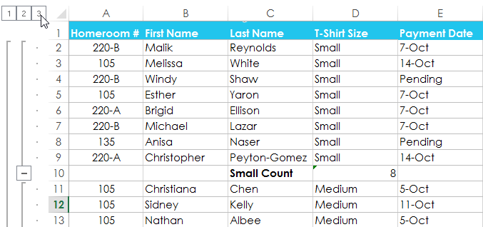 Viewing data at the highest level
You can also use the Show and Hide Detail buttons to show and hide the groups within the outline.
 Showing and hiding the new groups within the outline
Sometimes you may not want to keep subtotals in your worksheet, especially if you want to reorganize data in different ways. If you no longer want to use subtotaling, you'll need remove it from your worksheet.
Clicking the Subtotal command 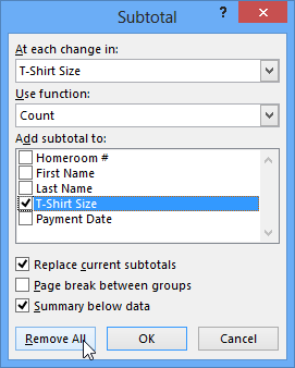 Removing subtotaling
To remove all groups without deleting the subtotals, click the Ungroup command drop-down arrow, then choose Clear Outline.
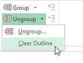 Removing all groups
/en/excel2013/tables/content/