
Excel 2013 -
Formatting Cells

Excel 2013
Formatting Cells

search
menu
/en/excel2013/modifying-columns-rows-and-cells/content/
All cell content uses the same formatting by default, which can make it difficult to read a workbook with a lot of information. Basic formatting can customize the look and feel of your workbook, allowing you to draw attention to specific sections and making your content easier to view and understand. You can also apply number formatting to tell Excel exactly what type of data you’re using in the workbook, such as percentages (%), currency ($), and so on
Optional: Download our practice workbook.
By default, the font of each new workbook is set to Calibri. However, Excel provides many other fonts you can use to customize your cell text. In the example below, we'll format our title cell to help distinguish it from the rest of the worksheet.
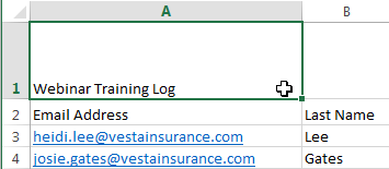 Selecting a cell
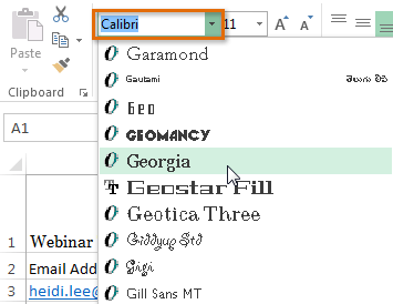 Choosing a font
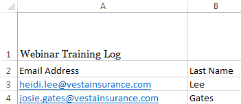 The new font
When creating a workbook in the workplace, you'll want to select a font that is easy to read. Along with Calibri, standard reading fonts include Cambria, Times New Roman, and Arial.
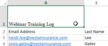 Selecting a cell
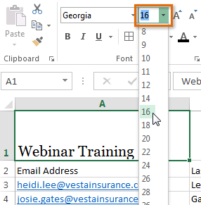 Choosing a new font size
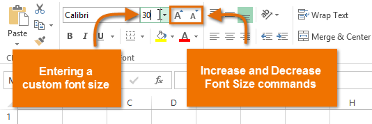
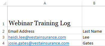 The new font size
You can also use the Increase Font Size and Decrease Font Size commands or enter a custom font size using your keyboard.
 Modifying the font size
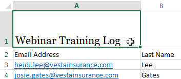 Selecting a cell
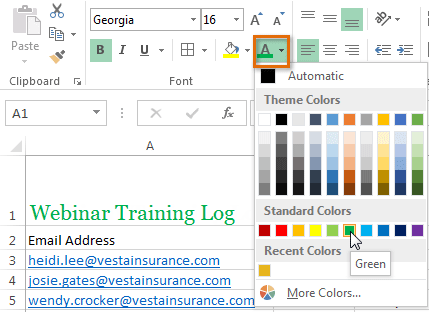 Choosing a font color
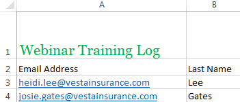 The new font color
Select More Colors at the bottom of the menu to access additional color options.
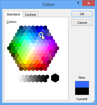 Selecting more colors
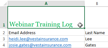 Selecting a cell
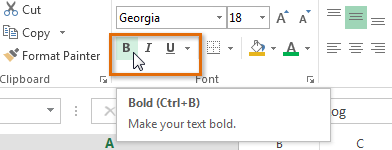 Clicking the Bold command
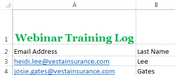 The bold text
You can also press Ctrl+B on your keyboard to make selected text bold, Ctrl+I to apply italics, and Ctrl+U to apply an underline.
By default, any text entered into your worksheet will be aligned to the bottom-left of a cell, while any numbers will be aligned to the bottom-right. Changing the alignment of your cell content allows you to choose how the content is displayed in any cell, which can make your cell content easier to read.
Click the arrows in the slideshow below to learn more about the different text alignment options.
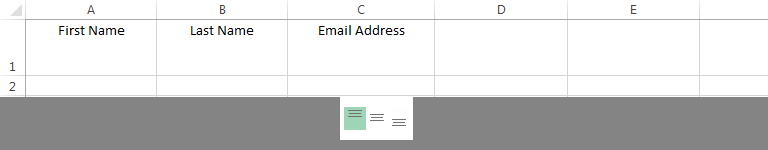
Left align: Aligns content to the left border of the cell
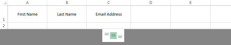
Center align: Aligns content an equal distance from the left and right borders of the cell
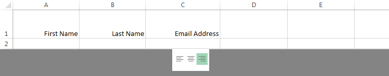
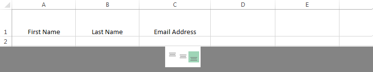
Right Align: Aligns content to the right border of the cell
Top Align: Aligns content to the top border of the cell
Middle Align: Aligns content an equal distance from the top and bottom borders of the cell
Bottom Align: Aligns content to the bottom border of the cell
In our example below, we'll modify the alignment of our title cell to create a more polished look and further distinguish it from the rest of the worksheet.
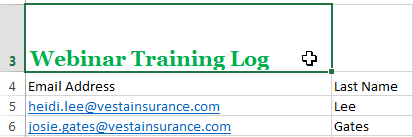 Selecting a cell
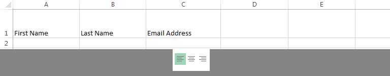
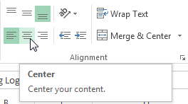 Choosing Center Align
 The realigned cell text
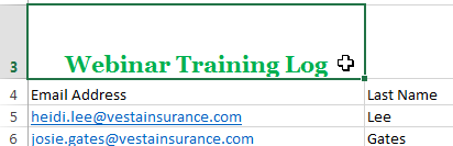 Selecting a cell
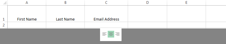
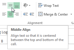 Choosing Middle Align
 The realigned cell text
You can apply both vertical and horizontal alignment settings to any cell.
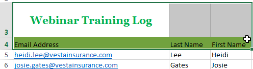
Cell borders and fill colors allow you to create clear and defined boundaries for different sections of your worksheet. Below, we'll add cell borders and fill color to our header cells to help distinguish them from the rest of the worksheet.
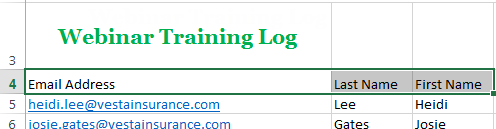 Selecting a cell range
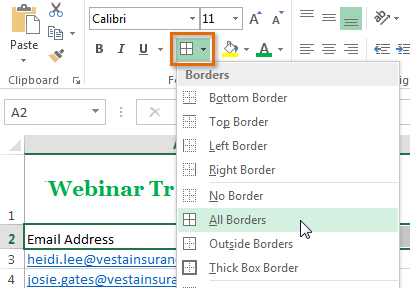 Choosing a border style
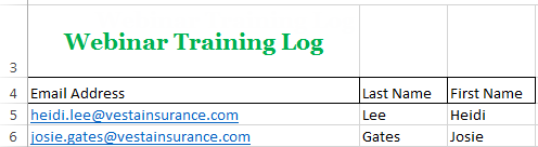 The added cell borders
You can draw borders and change the line style and color of borders with the Draw Borders tools at the bottom of the Borders drop-down menu.
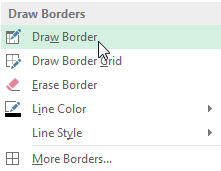 Drawing custom borders
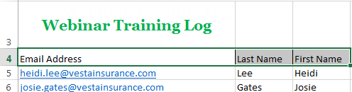 Selecting a cell range
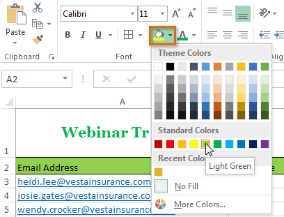 Choosing a cell fill color
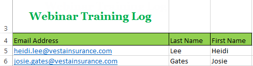 The new fill color
If you want to copy formatting from one cell to another, you can use the Format Painter command on the Home tab. When you click the Format Painter, it will copy all of the formatting from the selected cell. You can then click and drag over any cells you want to paste the formatting to.
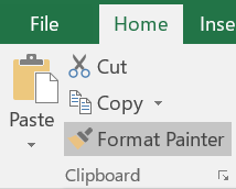
Watch the video below to learn two different ways to use the Format Painter.
Instead of formatting cells manually, you can use Excel's predesigned cell styles. Cell styles are a quick way to include professional formatting for different parts of your workbook, such as titles and headers.
In our example, we'll apply a new cell style to our existing title and header cells.
 Selecting a cell range
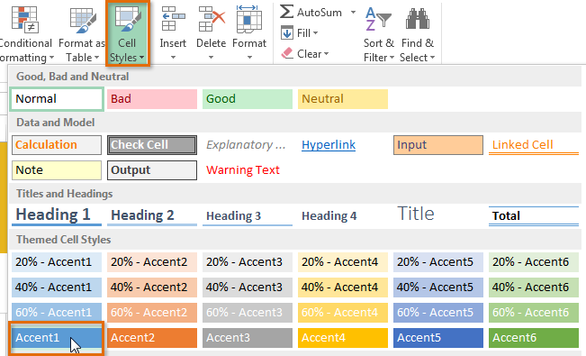 Choosing a cell style
 The new cell style
Applying a cell style will replace any existing cell formatting except for text alignment. You may not want to use cell styles if you've already added a lot of formatting to your workbook.
One of the most powerful tools in Excel is the ability to apply specific formatting for text and numbers. Instead of displaying all cell content in exactly the same way, you can use formatting to change the appearance of dates, times, decimals, percentages (%), currency ($), and much more.
In our example, we'll change the number format for several cells to modify the way dates are displayed.
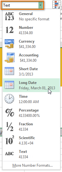 Choosing Long Date
 Click the buttons in the interactive below to learn about different text and number formatting options.

/en/excel2013/worksheet-basics/content/