
Excel 2010 -
Worksheet Basics

Excel 2010
Worksheet Basics

search
menu
/en/excel2010/creating-simple-formulas/content/
Every Excel workbook contains at least one or more worksheets. If you are working with a large amount of related data, you can use worksheets to help organize your data and make it easier to work with.
In this lesson, you will learn how to name and add color to worksheet tabs, as well as how to add, delete, copy, and move worksheets. Additionally, you will learn how to group and ungroup worksheets and freeze columns and rows in worksheets so they remain visible even when you're scrolling.
When you open an Excel workbook, there are three worksheets by default. The default names on the worksheet tabs are Sheet1, Sheet2, and Sheet3. To organize your workbook and make it easier to navigate, you can rename and even color code the worksheet tabs. Additionally, you can insert, delete, move, and copy worksheets.
Optional: You can download this example for extra practice.
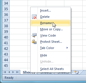 Selecting the Rename command
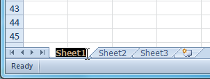 Renaming the worksheet
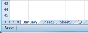 Renamed worksheet
Click the Insert Worksheet icon. A new worksheet will appear.
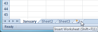 Inserting a new worksheet
You can change the setting for the default number of worksheets that appear in Excel workbooks. To access this setting, go into Backstage view and click Options.
Worksheets can be deleted from a workbook, including those containing data.
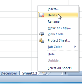 Deleting a worksheet
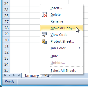 Selecting the Move or Copy command
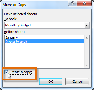 Checking the Create a copy box
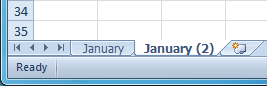 Copied worksheet
 .
.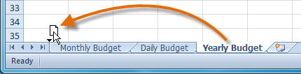 Moving a worksheet
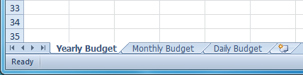 Moved worksheet
You can color worksheet tabs to help organize your worksheets and make your workbook easier to navigate.
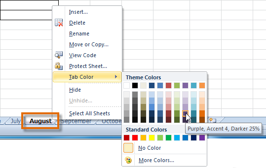 Changing the worksheet tab color
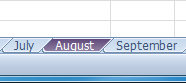 Worksheet tab color changed
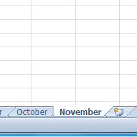
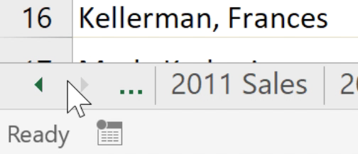
If you want to view a different worksheet, you can simply click the tab to switch to that worksheet. However, with larger workbooks this can sometimes become tedious, as it may require scrolling through all of the tabs to find the one you want. Instead, you can simply right-click the scroll arrows in the lower-left corner, as shown below.
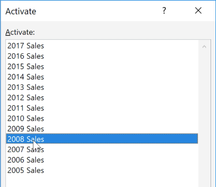
A dialog box will appear with a list of all of the sheets in your workbook. You can then double-click the sheet you want to jump to.
Watch the video below to see this shortcut in action.
You can work with each worksheet in a workbook individually, or you can work with multiple worksheets at the same time. Worksheets can be combined into a group. Any changes made to one worksheet in a group will be made to every worksheet in the group.
 Selecting the first worksheet to group
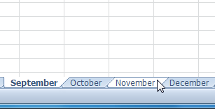 Selecting additional worksheets to group
While worksheets are grouped, you can navigate to any worksheet in the group and make changes that will appear on every worksheet in the group. If you click a worksheet tab that's not in the group, however, all of your worksheets will become ungrouped. You will have to group them again.
The ability to freeze specific rows or columns in your worksheet can be a useful feature in Excel. It is called freezing panes. When you freeze panes, you select rows or columns that will remain visible all the time, even as you are scrolling. This is particularly helpful when working with large spreadsheets.
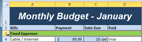 Selecting row 3
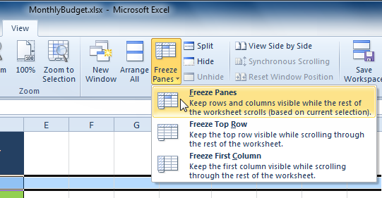 Selecting the Freeze Panes command from the View tab
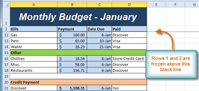 Rows 1 and 2 are frozen
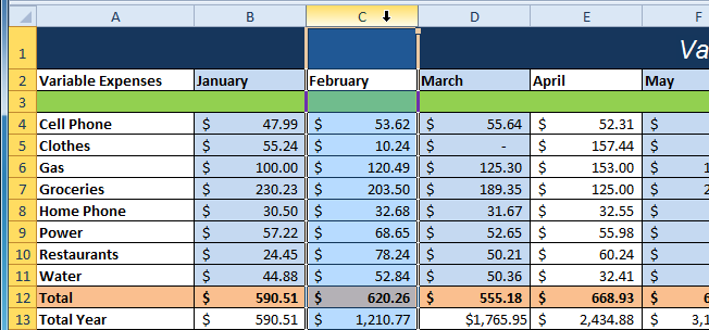 Selecting column C
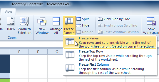 Selecting the Freeze Panes command from the View tab
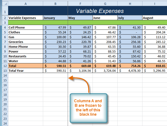 Columns A and B are frozen
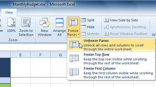 Selecting the Unfreeze Panes command from the View tab
/en/excel2010/printing/content/