
Excel 2010 -
Using Conditional Formatting

Excel 2010
Using Conditional Formatting

search
menu
/en/excel2010/working-with-sparklines/content/
Let's say you have a spreadsheet with thousands of rows of data. It would be extremely difficult to see patterns and trends just from examining the raw data. Excel gives us several tools that will make this task easier. One of these tools is called conditional formatting. With conditional formatting, you can apply formatting to one or more cells based on the value of the cell. You can highlight interesting or unusual cell values, and visualize the data using formatting such as colors, icons, and data bars.
In this lesson, you'll learn how to apply, modify, and remove conditional formatting rules.
Conditional formatting applies one or more rules to any cells you want. An example of a rule might be If the value is greater than 5000, color the cell yellow. By applying this rule to the cells in a worksheet, you'll be able to see at a glance which cells are more than 5000. There are also rules that can mark the top 10 items, all cells that are below the average, cells that are within a certain date range, and many more.
Optional: You can download this example for extra practice.
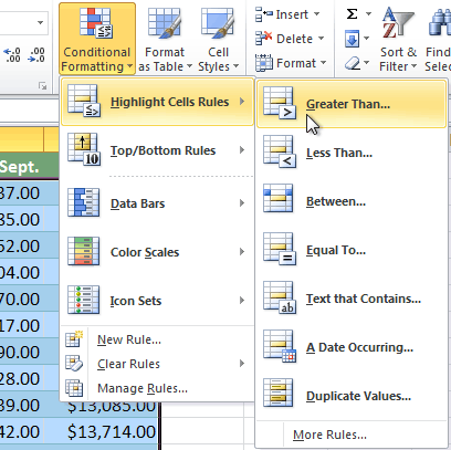 Selecting the Greater Than rule
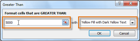 Entering a value and formatting style
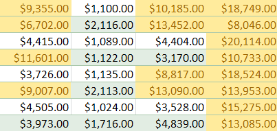 The formatted cells
If you want, you can apply more than one rule to your cells.
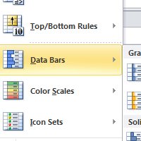
Excel has several presets you can use to quickly apply conditional formatting to your cells. They are grouped into three categories:
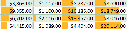 Data Bars
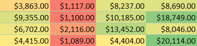 Color Scales
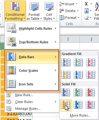 Selecting a formatting presetThe finished Data Bars
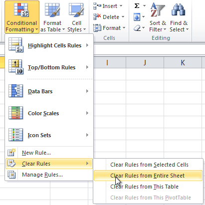 Clearing Rules
You can edit or delete individual rules by clicking the Conditional Formatting command and selecting Manage Rules. This is especially useful if you have applied multiple rules to the cells.
/en/excel2010/creating-pivottables/content/