Introduction

By the end of this lesson, you should be able to:

• Understand the definition of a function
• Use Excel 2003 functions in calculations
• Access Excel 2003 functions
• Find the sum of a range of data

Using functions

A function is a predefined formula that helps perform common mathematical functions. Functions save you the time of writing lengthy formulas. You could use an Excel function called Average, for example, to quickly find the average of range of numbers. Or you could use the Sum function to find the sum of a cell range. Excel 2003 contains many different functions.

Each function has a specific order, called syntax, which must be strictly followed for the function to work correctly.

Syntax order:

1. All functions begin with the = sign.
2. After the = sign, define the function name (e.g., Sum).
3. Add one or more arguments—numbers, text, or cell references—enclosed by parentheses. If there is more than one argument, separate each by a comma.

An example of a function with one argument that adds a range of cells, B3 through B10:

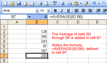
An example of a function with more than one argument that calculates the average of numbers in a range of cells, B3 through B10 and C3 through C10:

Excel literally has hundreds of different functions to assist with your calculations. Building formulas can be difficult and time consuming. Excel's functions can save you a lot of time and headaches.

Excel's different functions

There are many different functions in Excel 2003. Some of the more common functions include:

Statistical functions:

• SUM: Summation adds a range of cells together.
• AVERAGE: Average calculates the average of a range of cells.
• COUNT: This counts the number of chosen data in a range of cells.
• MAX: This identifies the largest number in a range of cells.
• MIN: This identifies the smallest number in a range of cells.

Financial functions:

• Interest rates
• Loan payments
• Depreciation amounts

Date and time functions:

• DATE: This converts a serial number to a day of the month.
• Day of Week
• DAYS360: This calculates the number of days between two dates based on a 360-day year.
• TIME: This returns the serial number of a particular time.
• HOUR: This converts a serial number to an hour.
• MINUTE: This converts a serial number to a minute.
• TODAY: This returns the serial number of today's date.
• MONTH: This converts a serial number to a month.
• YEAR: This converts a serial number to a year.

You don't have to memorize these functions, but you should have an idea of what each can do for you.

Finding the sum of a range of data

The AutoSum function allows you to create a formula that includes a cell range—many cells in a column, for example, or many cells in a row.

To calculate the AutoSum of a range of data:

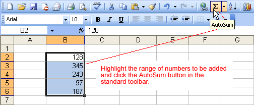
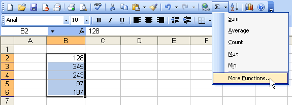
• Type the numbers to be included in the formula in separate cells of column B (type 128 in cell B2, 345 in cell B3, 243 in cell B4, 97 in cell B5, and 187 cell B6).
• Click the first cell (B2) to be included in the formula.
• Using the point-click-drag method, drag the mouse to define a cell range from cell B2 through cell B6.
• On the Standard toolbar, click the Sum button.
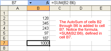
• The sum of the numbers is added to cell B7, or the cell immediately beneath the defined range of numbers.
• Notice the formula, =SUM(B2:B6), has been defined to cell B7.
  
  

Finding the average of a range of numbers

The Average function calculates the average of a range of numbers. The Average function can be selected from the AutoSum drop-down menu.

To calculate the average of a range of data:

• Type the numbers to be included in the formula in separate cells of column B (type 128 in cell B2, 345 in cell B3, 243 in cell B4, 97 in cell B5, and 187 cell B6).
• Click the first cell (B2) to be included in the formula.
• Using the point-click-drag method, drag the mouse to define a cell range from cell B2 through cell B6.
• On the Standard toolbar, click on the drop-down part of the AutoSum button.
  
  
• Select the Average function from the drop-down Functions list.
  
  
• The average of the numbers is added to cell B7, or the cell immediately beneath the defined range of numbers.
• Notice the formula, =AVERAGE(B2:B6), has been defined to cell B7.
  
  

Accessing Excel 2003 functions

To access other functions in Excel:

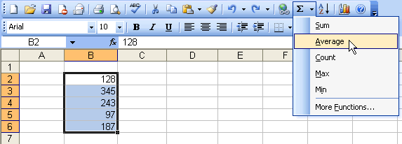
• Using the point-click-drag method, select a cell range to be included in the formula.
• On the Standard toolbar, click on the drop-down part of the AutoSum button.
• If you don't see the function you want to use (Sum, Average, Count, Max, Min), display additional functions by selecting More Functions.
  
  
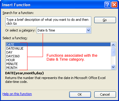
• The Insert Function dialog box opens.
• There are three ways to locate a function in the Insert Function dialog box:

You can type a question in the Search for a function box and click GO.

You can scroll through the alphabetical list of functions in the Select a function field.

You can select a function category in the Select a category drop-down list and review the corresponding function names in the Select a function field.

• Select the function you want to use, then click the OK button.

If you're comfortable with basic functions, you may want to try a more advanced one like VLOOKUP. You can check out our article on How to Use Excel's VLOOKUP Function for more information. If you want to learn even more about functions, check out our Excel Formulas tutorial.

Challenge!

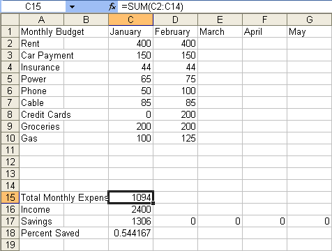
• Open your Monthly Budget file.
• Type the following in Row 1:
  • February in D1
  • March in E1
  • April in F1
  • May in G1
  • June in H1
  • July in I1
  • August in J1
  • September in K1
  • October in L1
  • November in M1
  • December in N1
  • Total in O1
• Type the amount of your expenses in each cell in Column D (cells 2 through 17), just like you did with Column C in a previous challenge.
• Delete the number in C15.
• Type a function in cell C15 that adds the range of cells: C2 through C14.
• Fill the formula from C15 to D15 through O15.
• Type your Income for the month of February in D16.
• Type a formula in O17 that adds your savings for the year. Because you have only entered data for the month of January and February, this amount indicates your savings for the two months.
• Save and close the Monthly Budget spreadsheet.