أكسيل 2016: (Cell References) مراجع الخلايا النسبية والمطلقة
5b63209b44ff9509105677445b63357344ff95091056776a
Lesson 15: (Cell References) مراجع الخلايا النسبية والمطلقة
/en/tr_ar-excel-2016/complex-formulas-/content/
المقدمة
There are two types of cell references: relative and absolute. Relative and absolute references behave differently when copied and filled to other cells. Relative references change when a formula is copied to another cell. Absolute references, on the other hand, remain constant no matter where they are copied.
Watch the video below to learn more about cell references.
Relative references
By default, all cell references are relative references. When copied across multiple cells, they change based on the relative position of rows and columns. For example, if you copy the formula =A1+B1 from row 1 to row 2, the formula will become =A2+B2. Relative references are especially convenient whenever you need to repeat the same calculation across multiple rows or columns.
To create and copy a formula using relative references:
In the following example, we want to create a formula that will multiply each item's price by the quantity. Instead of creating a new formula for each row, we can create a single formula in cell D2 and then copy it to the other rows. We'll use relative references so the formula calculates the total for each item correctly.
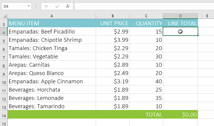
Select the cell that will contain the formula. In our example, we'll select cell D4.
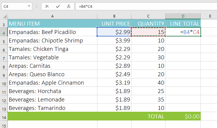
Enter the formula to calculate the desired value. In our example, we'll type =B4*C4.
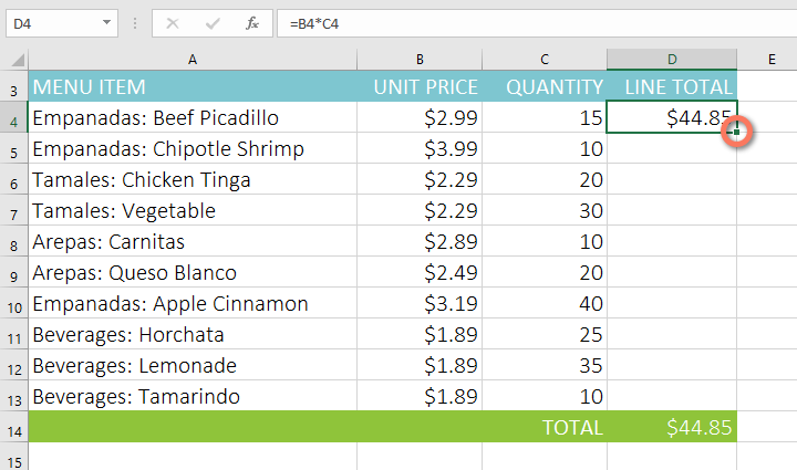
Press Enter on your keyboard. The formula will be calculated, and the result will be displayed in the cell.
Locate the fill handle in the bottom-right corner of the desired cell. In our example, we'll locate the fill handle for cell D4.
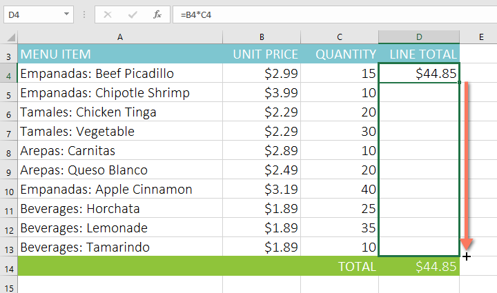
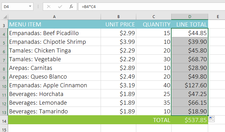
Click and drag the fill handle over the cells you want to fill. In our example, we'll select cells D5:D13.
Release the mouse. The formula will be copied to the selected cells with relative references, displaying the result in each cell.
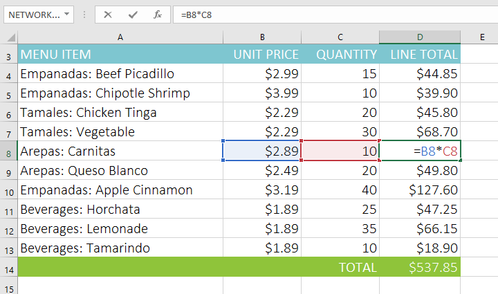
You can double-click the filled cells to check their formulas for accuracy. The relative cell references should be different for each cell, depending on their rows.
Absolute references
There may be a time when you don't want a cell reference to change when copied to other cells. Unlike relative references, absolute references do not change when copied or filled. You can use an absolute reference to keep a row and/or column constant.
An absolute reference is designated in a formula by the addition of a dollar sign ($). It can precede the column reference, the row reference, or both.
You will generally use the $A$2 format when creating formulas that contain absolute references. The other two formats are used much less frequently.
When writing a formula, you can press the F4 key on your keyboard to switch between relative and absolute cell references. This is an easy way to quickly insert an absolute reference.
To create and copy a formula using absolute references:
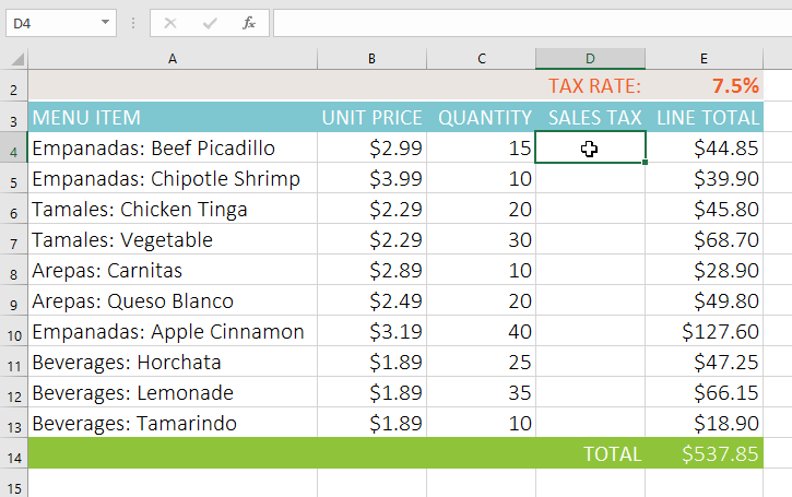
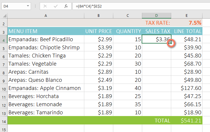
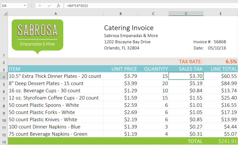
In the example below, we're going to use cell E2 (which contains the tax rate at 7.5%) to calculate the sales tax for each item in column D. To make sure the reference to the tax rate stays constant, even when the formula is copied and filled to other cells, we'll need to make cell $E$2 an absolute reference.
Select the cell that will contain the formula. In our example, we'll select cell D4.
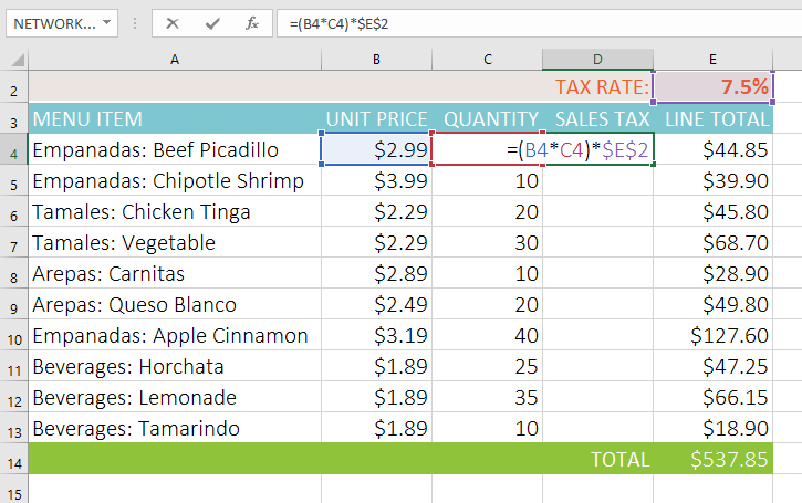
Enter the formula to calculate the desired value. In our example, we'll type =(B4*C4)*$E$2, making $E$2 an absolute reference.
Press Enter on your keyboard. The formula will calculate, and the result will display in the cell.
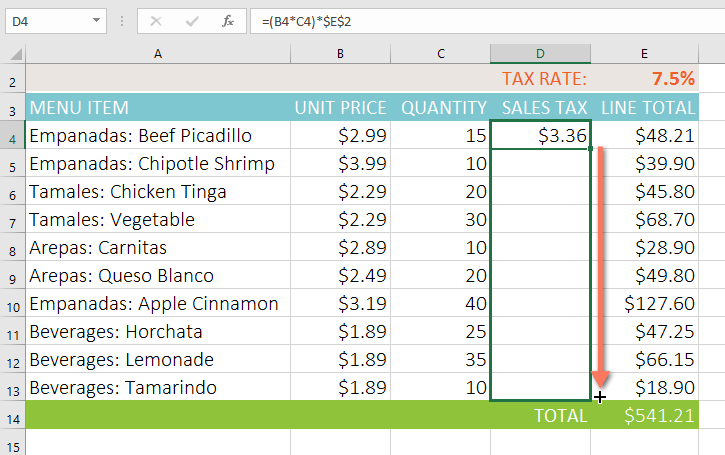
Locate the fill handle in the bottom-right corner of the desired cell. In our example, we'll locate the fill handle for cell D4.
Click and drag the fill handle over the cells you want to fill (cells D5:D13 in our example).
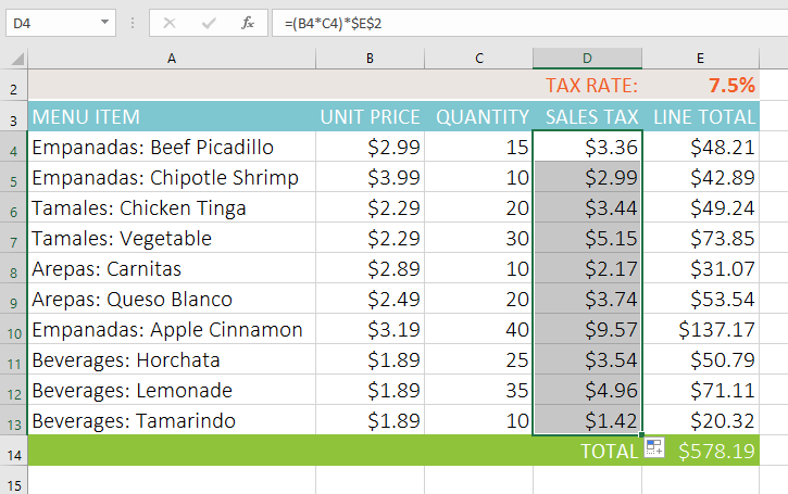
Release the mouse. The formula will be copied to the selected cells with an absolute reference, and the values will be calculated in each cell.
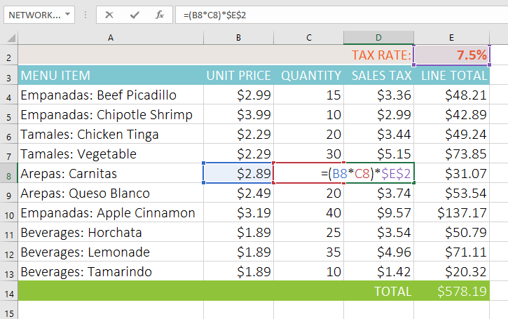
You can double-click the filled cells to check their formulas for accuracy. The absolute reference should be the same for each cell, while the other references are relative to the cell's row.
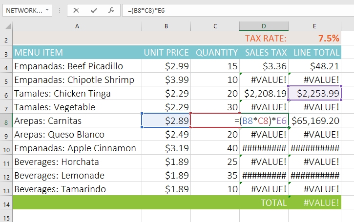
Be sure to include the dollar sign ($) whenever you're making an absolute reference across multiple cells. The dollar signs were omitted in the example below. This caused Excel to interpret it as a relative reference, producing an incorrect result when copied to other cells.
Using cell references with multiple worksheets
Excel allows you to refer to any cell on any worksheet, which can be especially helpful if you want to reference a specific value from one worksheet to another. To do this, you'll simply need to begin the cell reference with the worksheet name followed by an exclamation point (!). For example, if you wanted to reference cell A1 on Sheet1, its cell reference would be Sheet1!4 امبير
Note that if a worksheet name contains a space, you'll need to include single quotation marks (' ') around the name. For example, if you wanted to reference cell A1 on a worksheet named July Budget, its cell reference would be 'July Budget'!4 امبير
To reference cells across worksheets:
In our example below, we'll refer to a cell with a calculated value between two worksheets. This will allow us to use the exact same value on two different worksheets without rewriting the formula or copying data.
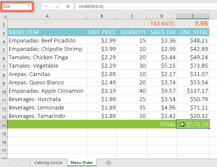
Locate the cell you want to reference, and note its worksheet. In our example, we want to reference cell E14 on the Menu Order worksheet.
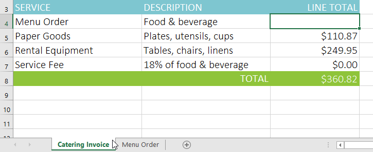
Navigate to the desired worksheet. In our example, we'll select the Catering Invoice worksheet.
Locate and select the cell where you want the value to appear. In our example, we'll select cell B4.
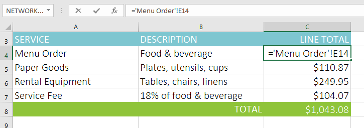
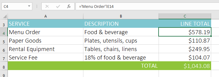
Type the equals sign (=), the sheet name followed by an exclamation point (!), and the cell address. In our example, we'll type ='Menu Order'!(ث)
Press Enter on your keyboard. The value of the referenced cell will appear. Now, if the value of cell E14 changes on the Menu Order worksheet, it will be updated automatically on the Catering Invoice worksheet.
If you rename your worksheet at a later point, the cell reference will be updated automatically to reflect the new worksheet name.
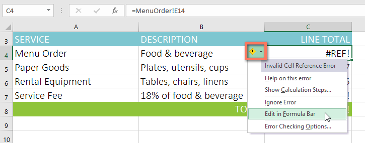
If you enter a worksheet name incorrectly, the #REF! error will appear in the cell. In our example below, we've mistyped the name of the worksheet. To edit, ignore, or investigate the error, click the Error button beside the cell and choose an option from the menu.
Click the Paper Goods tab in the bottom-left of the workbook.
In cell D4, enter a formula that multiplies the unit price in B4, the quantity in C4, and the tax rate in E2. Make sure to use an absolute cell reference for the tax rate because it will be the same in every cell.
Use the fill handle to copy the formula you just created to cells D5:D12.
Change the tax rate in cell E2 to 6.5%. Notice that all of your cells have updated. When you're finished, your workbook should look like this:
Click the Catering Invoice tab.
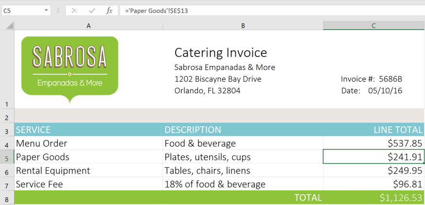
Delete the value in cell C5 and replace it with a reference to the total cost of the paper goods. Hint: The cost of the paper goods is in cell E13 on the Paper Goods worksheet.
Optional: Use the same steps from above to calculate the sales tax for each item on the Menu Order worksheet. The total cost in cell E14 should update. Then, in cell C4 of the Catering Invoice worksheet, create a cell reference to the total you just calculated. Note: If you used our practice workbook to follow along during the lesson, you may have already completed this step.
When you're finished, your workbook should look something like this: